Answer to Question #135359 in Statistics and Probability for Sana

Question

You have to examine the relationship between the age and price for used cars
sold in the last year by a car dealership company. Fit a simple linear regression
model Price Sold on Car age.
(b) Find the estimated linear regression values of Y.
(c) Show that the sum of Deviations of estimated values from actual values is
zero.
(d) Show that the sum of squares of residuals is minimum.
(e) Find the standard error of estimate. Calculate the Correlation Co-efficient y on x.
(g) Find the Co-efficient of Determination.
Car Age (in years) Price (in dollars)
4 6300
4 5800
5 5700
5 4500
7 4500
7 4200
8 4100
9 3100
10 2100
11 2500
12 2200

Answer 1

$\begin{matrix} & x & y & xy & x^2 & y^2 \\ & 4 & 6300 & 25200 & 16 & 39690000 \\ & 4 & 5800 & 23200 & 16 & 33640000 \\ & 5 & 5700 & 28500 & 25 & 32490000 \\ & 5 & 4500 & 22500 & 25 & 20250000 \\ & 7 & 4500 & 31500 & 49 & 20250000 \\ & 7 & 4200 & 29400 & 49 & 17640000 \\ & 8 & 4100 & 32800 & 64 & 16810000\\ & 9 & 3100 & 27900 & 81 & 9610000 \\ & 10 & 2100 & 21000 & 100 & 4410000 \\ & 11 & 2500 & 27500 & 121 & 6250000 \\ & 12 & 2200 & 26400 & 144 & 4840000 \\ Sum= & 82 & 45000 & 265900 & 690 & 205880000 \end{matrix}$

$\bar{x}=\dfrac{1}{n}\displaystyle\sum_{i=1}^nx_i=\dfrac{82}{11}\approx7.454545$

$\bar{y}=\dfrac{1}{n}\displaystyle\sum_{i=1}^ny_i=\dfrac{45000}{11}\approx40.909091$

$SS_{xx}=\displaystyle\sum_{i=1}^nx_i^2-\dfrac{1}{n}(\displaystyle\sum_{i=1}^nx_i)^2=$

$=690-\dfrac{82^2}{11}\approx78.727273$

$SS_{yy}=\displaystyle\sum_{i=1}^ny_i^2-\dfrac{1}{n}(\displaystyle\sum_{i=1}^ny_i)^2=$

$=205880000 -\dfrac{45000^2}{11}\approx21789090.909091$

$SS_{xy}=\displaystyle\sum_{i=1}^nx_iy_i-\dfrac{1}{n}(\displaystyle\sum_{i=1}^nx_i)(\displaystyle\sum_{i=1}^ny_i)=$

$=265900 -\dfrac{82\cdot45000}{11}\approx-39554.545455$

Therefore, based on the above calculations, the regression coefficients (the slope $m,$

and the y-intercept $n$) are obtained as follows:

$m=\dfrac{SS_{xy}}{SS_{xx}}\approx-502.424942$

$n=\bar{y}-m\cdot\bar{x}\approx$

$\approx40.909091-(-502.424942)\cdot7.454545\approx7836.25866$

Therefore, we find that the regression equation is:

$y=7836.25866-502.424942x$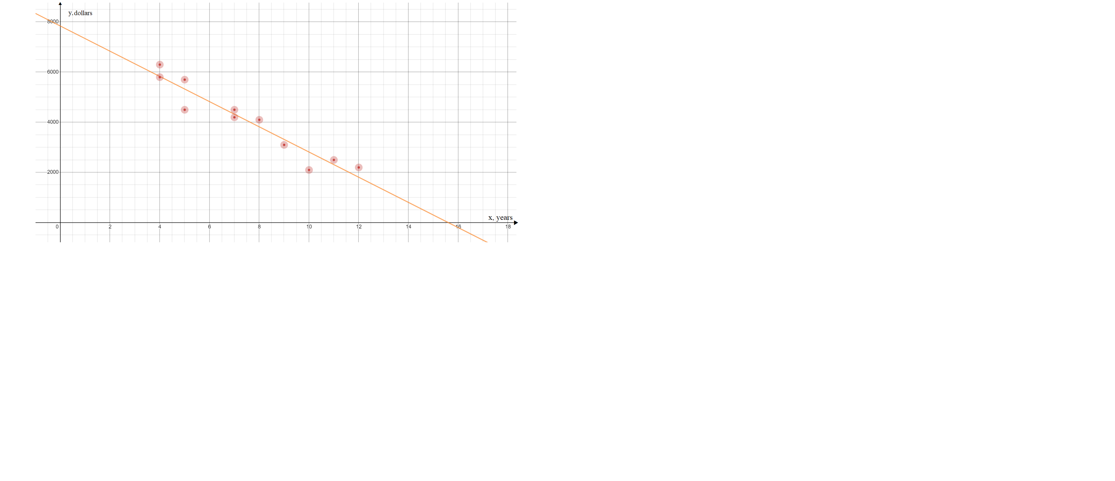

$y(4)=7836.25866-502.424942(4)=5826.56$

$y(5)=7836.25866-502.424942(5)=5324.13$

$y(7)=7836.25866-502.424942(7)=4319.28$

$y(8)=7836.25866-502.424942(8)=3816.86$

$y(9)=7836.25866-502.424942(9)=3314.43$

$y(10)=7836.25866-502.424942(10)=2812.01$

$y(11)=7836.25866-502.424942(11)=2309.58$

$y(12)=7836.25866-502.424942(12)=1807.16$

$6300-5826.56+5800-5826.56+$ $+5700-5324.13+4500-5324.13+$ $+4500-4319.28+4200-4319.28+$ $+4100-3816.86+3100-3314.43+$ $+2100-2812.01+2500-2309.58+$ $+2200-1807.16=0.02\approx0$

$RSS=\displaystyle\sum_{i=1}^n(y_{iobs}-y_{ipred})^2=SS_{yy}-mSS_{xy}=$

$=SS_{yy}(1-\dfrac{SS_{xy}^2}{SS_{xx}SS_{yy}})=$

$=21789090.909091(1-\dfrac{(-39554.545455)^2}{78.727273(21789090.909091)})=$

$=1915896.5844$

The sum of square of residuals is minimum for points lying on the regression line and so cannot be less than $1915896.5844$ for any other line.

$s_{est}=\sqrt{\dfrac{RSS}{n-2}}\approx\sqrt{\dfrac{1915896.5844}{11-2}}\approx461.39$

$r=\dfrac{SS_{xy}}{\sqrt{SS_{xx}}\sqrt{SS_{yy}}}=\dfrac{-39554.545455}{\sqrt{78.727273}\sqrt{21789090.909091}}\approx$

$\approx-0.955024$

Strong negarive correlation.

$r^2\approx0.912071$