Question

A system is known whose input - output relationship is determined by the following difference equation :

y(n)-1/2y(n-1)=x(n)+1/2x(n-1)

Find the system function H ( z ) and plot the pole - zero plot

Answer 1

In the general case, the representation of a linear system using a linear difference equation with constant coefficients

$$\sum_{i=0}^N a_i y[n-i]=\sum_{j=0}^M b_j x[n-j]$$

Taking the Z-transform of the equation (using linearity and time-shifting laws) yields

$$Y(z)\sum_{i=0}^N a_i z^{-i}=X(z)\sum_{j=0}^M b_j z^{-j}$$

reordering the result gives a transfer function

$$H(z)=\frac{Y(z)}{X(z)}=\frac{\sum_{j=0}^M b_j z^{-j}}{\sum_{i=0}^N a_i z^{-i}}=\frac {b_0 +b_1 z^{-1}+...+b_M z^{-M}}{a_0 +a_1 z^{-1}+...+a_Nz^{-N}}$$

where the numerator has M roots (corresponding to zeros of H) and the denominator has N roots (corresponding to poles of H)

Zeros and poles are usually complex, and in order to plot them on the complex plane (pole-zero plot) we rewrite the transfer function in terms of zeros and poles

$$H(z)=\frac {b_0 +b_1 z^{-1}+...+b_M z^{-M}}{a_0 +a_1 z^{-1}+...+a_Nz^{-N}}=\frac{(1-q_1 z^{-1})(1-q_2 z^{-1})...(1-q_M z^{-1})}{(1-p_1 z^{-1})(1-p_2 z^{-1})...(1-p_N z^{-1})}$$

where q_k is the k-th zero and p_k is the k-th pole.

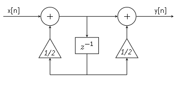
So, if the linear difference equation

$$y[n]-\frac 1 2 y[n-1]=x[n]+\frac 1 2 x[n-1]$$

where

$$M=N=1,\space a_0=b_0=1, \space a_1 =-\frac 1 2, \space b_1=\frac 1 2$$

Then the transfer function is

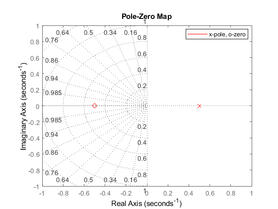
$$H(z)=\frac{Y(z)}{X(z)}=\frac{b_0+b_1 z^{-1}}{a_0+a_1 z^{-1}}=\frac {1+\frac 1 2 z^{-1}}{1-\frac 1 2 z^{-1}}$$

the numerator has root (corresponding to zero of H)

$$q_1 =-\frac 1 2$$

the denominator has root (corresponding to pole of H)

$$p_1=\frac 1 2$$

The DT LTI system

The pole-zero plot